Euler Approximation Project

Dennis O'Connell

06/05/2020

Problem 1

The non-linear initial value problem in question is the following: $$y^{\prime}=5-3 \sqrt{y}, \quad y(0)=2$$ Our goal is to compute approximate values to the equation at the points $$t=0.5,1,1.5,2.0,2.5$$ and plot solutions using: $$a)\: h=0.1 \: b)\: h=0.05\: c)\: h=0.025 \: d)\: h=0.01$$

Part A) h=.1

The Euler's method states that $$y_{n+1}=y_{n}+h \cdot f\left(t_{n}, y_{n}\right),$$ where $$t_{n+1}=t_{n}+h$$

When h=.1 and t=.5 we have that $$h=\frac{1}{10}, t_{0}=0, y_{0}=2, f(t, y)=5-3 \sqrt{y}$$ We have a step size of .1 and we are trying to approximate y(.5) so we will use this method to calculate one point at each of the five steps

Step 1

$$\begin{array}{l} t_{1}=t_{0}+h=0+\frac{1}{10}=\frac{1}{10} \\ y\left(t_{1}\right)=y\left(\frac{1}{10}\right)=y_{1}=y_{0}+h \cdot f\left(t_{0}, y_{0}\right)=2+h \cdot f(0,2)= \\ =2+\frac{1}{10} \cdot(0.757359312880715)=2.07573593128807 \end{array}$$

Step 2

$$\begin{array}{l} t_{2}=t_{1}+h=\frac{1}{10}+\frac{1}{10}=\frac{1}{5} \\ y\left(t_{2}\right)=y\left(\frac{1}{5}\right)=y_{2}=y_{1}+h \cdot f\left(t_{1}, y_{1}\right)=2.07573593128807+h \\ \cdot f\left(\frac{1}{10}, 2.07573593128807\right)= \\ =2.07573593128807+\frac{1}{10} \cdot(0.677775644232169)=2.14351349571129 \end{array}$$

Step 3

$$\begin{array}{l} t_{3}=t_{2}+h=\frac{1}{5}+\frac{1}{10}=\frac{3}{10} \\ y\left(t_{3}\right)=y\left(\frac{3}{10}\right)=y_{3}=y_{2}+h \cdot f\left(t_{2}, y_{2}\right)=2.14351349571129+h \\ \cdot f\left(\frac{1}{5}, 2.14351349571129\right)= \\ =2.14351349571129+\frac{1}{10} \cdot(0.607777161686625)=2.20429121187995 \end{array}$$

Step 4

$$\begin{array}{l} t_{4}=t_{3}+h=\frac{3}{10}+\frac{1}{10}=\frac{2}{5} \\ y\left(t_{4}\right)=y\left(\frac{2}{5}\right)=y_{4}=y_{3}+h \cdot f\left(t_{3}, y_{3}\right)=2.20429121187995+h \\ \cdot f\left(\frac{3}{10}, 2.20429121187995\right)= \\ =2.20429121187995+\frac{1}{10} \cdot(0.545943320194549)=2.25888554389941 \end{array}$$

Step 5

$$\begin{array}{l} t_{5}=t_{4}+h=\frac{2}{5}+\frac{1}{10}=\frac{1}{2} \\ y\left(t_{5}\right)=y\left(\frac{1}{2}\right)=y_{5}=y_{4}+h \cdot f\left(t_{4}, y_{4}\right)=2.25888554389941+h \\ \cdot f\left(\frac{2}{5}, 2.25888554389941\right)= \\ =2.25888554389941+\frac{1}{10} \cdot(0.491123211364648)=2.30799786503587 \\ \end{array}$$

Answer

$$y\left(\frac{1}{2}\right)=2.30799786503587$$

Now repeat the process for t=1

This time we have 10 steps since there are ten steps of length .1 in t=1. After computations we get the approximation $$y(1)=2.49006201824323$$

Keep repeating the process for t=1.5,2.0,2.5

$$y\left(\frac{3}{2}\right)=2.60022620250401$$ $$y(2)=2.66772787250012$$ $$y\left(\frac{5}{2}\right)=2.70938800499274$$

Part B) h=.05

This time we will see twice as many steps as there were in part a because the step size has been reduced by a half

When h=.05 and t=.05, we have $$h=\frac{1}{20}, t_{0}=0, y_{0}=2, f(t, y)=5-3 \sqrt{y}$$ Now use Euler's method to approximate y(.5) after 10 steps

Answer

$$y\left(\frac{1}{2}\right)=2.30166603354356$$

Just like in Part A, we repeat this process for T=1,1.5,2.0,2.5

Answers

$$y(1)=2.48262624738228$$ $$y\left(\frac{3}{2}\right)=2.59351710664336$$ $$y(2)=2.6622699286492$$ $$y\left(\frac{5}{2}\right)=2.70518844985266$$

Part C)

h=0.025

Answers

$$y\left(\frac{1}{2}\right)=2.29863798427263$$ $$y(1)=2.47902957749642$$ $$y\left(\frac{3}{2}\right)=2.59023973355631$$ $$y(2)=2.65957929689476$$ $$y\left(\frac{5}{2}\right)=2.70310002326473$$

Part D)

h=0.01

Answers

$$y\left(\frac{1}{2}\right)=2.29686258733234$$ $$y(1)=2.47690855658606$$ $$y\left(\frac{3}{2}\right)=2.58829723261312$$ $$y(2)=2.65797708416176$$ $$y\left(\frac{5}{2}\right)=2.70310002326473$$

Interactive Plot

h1=> h=.1

h2=> h=.05

h3=> h=.025

h4=> h=.01

Comments on the behavior

With smaller values of h, it seems that our answers are becoming more refined and closer to a single solution. Though it is difficult to see on the interactive graph, the approximations at h=.01 are closer to a single solution than they are at h=.1

Problem 2

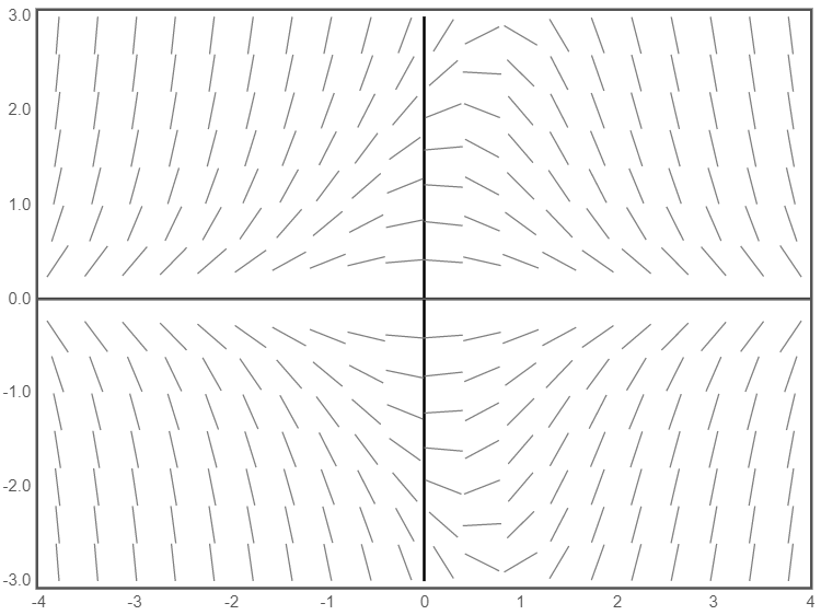
In this problem, we are concerned with the following initial value problem: $$y^{\prime}=-t y+0.1 y^{3}, \quad y(0)=\alpha$$

This differential equation can be represented by the vector field below:

Part A

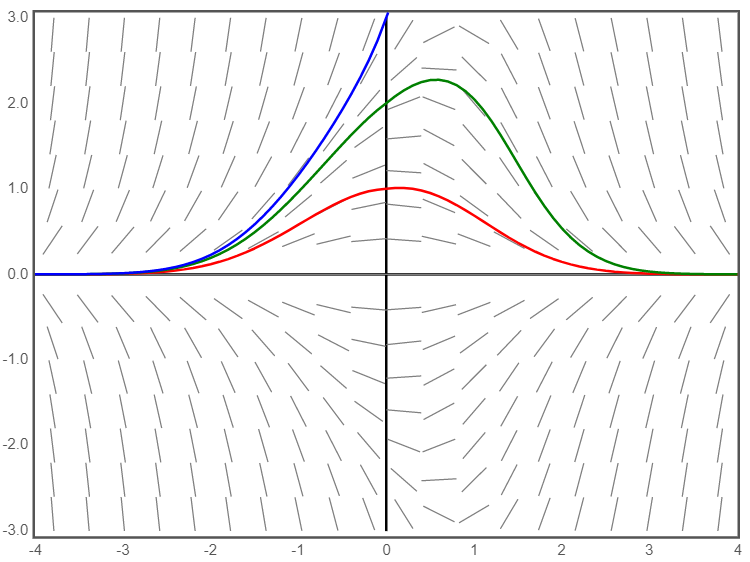
When we plug in different values for alpha between 1 and 4 we get lines of different behaviors

The red line represents alpha = 1

The green line represents alpha = 2

The blue line represents alpha = 3

It is clear that between alpha = 2 and alpha = 3, there is a value for alpha that is a "tipping point" that leads to either divergence or convergence.

Part B

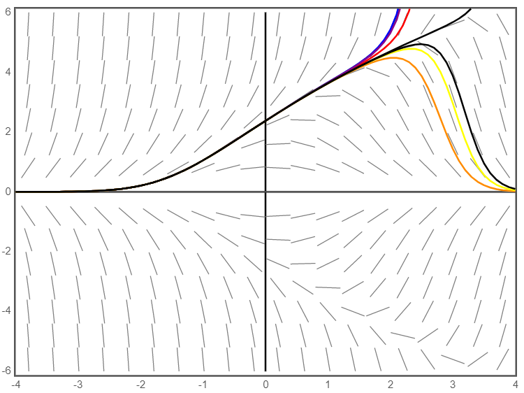
In order to approximate the value of this tipping point, I plugged in values of alpha between 2 and 3 until they either drew a line that diverged or converged.

Last black line is alpha = 2.3714, it seems that the tipping point is about 2.73

Here, each time that I plugged in a value for alpha with a decimal place that was either slightly greater than 2.3 and if it stayed convergent then I would keep on increasing the value of the decimal place until it became divergent.

Part C

In order to approximate the tipping point, we can also use Euler's method

With h=.01, we get

$$y\left(\frac{1}{2}\right)=3.01399704820084$$ $$y(1)=3.58697080063328$$ $$y\left(\frac{3}{2}\right)=3.96777080880568$$ $$y(2)=3.50207152939925$$

Technologies used for this project

Emathhelp.net was used for performing the computations of each Euler approximation. Link.

D3, a javascript datavisualization library, was used to plot the points created by each approximation in problem 1. Link.

Darryl Nester's Slope Field Generator was used to calculate the slope field of the differntial equation in problem two. Link.

Mathjax was used to render the LaTeX on this webpage. Link.

Lastly, Bootstrap was used for styling.

Check out the Github Repo here: Link.